ACTIVE · shadyknollcave.io

SPECTRA

Spatial Platform for Efficient Cloud Tile Raster Access

Zero-copy inference  ·  Accelerated mission detection  ·  Cloud-Native Geospatial Intelligence

scroll

Three primitives.
Infinite scale.

SPECTRA is built on open geospatial standards — no proprietary lock-in, no monolithic servers, no pre-tiling marathons.

🗂
stac 1.0

SpatioTemporal Asset Catalog

A universal language for geospatial data. Every image is a STAC Item — a JSON record with geometry, datetime, and typed asset links (raw JPG, ortho thumbnail, COG). Catalogs are static JSON files served from any CDN, consumed by any compliant viewer.

Open Catalog →
🌐
COG · GeoTIFF

Cloud Optimized GeoTIFF

GeoTIFFs engineered for HTTP range requests. Internal tiling + overviews mean a client fetches only the pixels it needs — a 512×512 chip from a 4000×3000 scene costs one round-trip. No preprocessing, no mosaic server, no waiting.

Inspect a COG →
TiTiler · FastAPI

Dynamic Tile Server

A FastAPI tile server that reads COGs on the fly. Pass any COG URL and get back XYZ tiles, bbox crops, previews, or band statistics — all computed from range-reads against the source file. Zero data duplication.

Browse the API →

From sensor to inference.

Every drone image flows through a deterministic pipeline: raw capture → metadata extraction → three published assets → on-demand chips → CV model.

🚁
Drone JPEG
raw · EXIF+XMP
📋
STAC Item
geo · datetime · assets
🗺
COG Assets
ortho · 4000×3000px
TiTiler
chip on demand
🤖
CV / YOLO
geo-registered output
inference_pipeline.py
# SPECTRA CV pipeline — loop the catalog, infer on every COG
import pystac, rasterio, numpy as np
from ultralytics import YOLO

# ── 1. load catalog (static JSON, no API server needed) ──────────────────
catalog = pystac.read_file("https://drone-catalog.shadyknollcave.io/catalog.json")
model   = YOLO("yolo11n.pt")

# ── 2. iterate items, range-read only the pixels we need ─────────────────
for item in catalog.get_all_items():
    cog_url = pystac.utils.make_absolute_href(
        item.assets["visual"].href,
        item.get_self_href()
    )
    with rasterio.open(cog_url) as ds:
        img       = ds.read([1,2,3]).transpose(1,2,0)  # (H,W,3) uint8
        transform = ds.transform  # affine: pixel → CRS coords

    # ── 3. run inference ─────────────────────────────────────────────────
    results = model(img)

    # ── 4. project detections back to WGS-84 ─────────────────────────────
    for box in results[0].boxes.xyxy.tolist():  # [x0,y0,x1,y1]
        x0, y0, x1, y1 = box
        # ds.xy(row, col) — note y=row, x=col
        lon0, lat0 = rasterio.transform.xy(transform, y0, x0)
        lon1, lat1 = rasterio.transform.xy(transform, y1, x1)
        print(f"bbox ({lon0:.6f},{lat0:.6f}) → ({lon1:.6f},{lat1:.6f})")

Every URL is a live query.

These are real HTTP calls — click any card to see TiTiler fetch and render a section of the drone COG in real time, using HTTP range requests.

COG Preview
PREVIEW

Full-scene overview

titiler.shadyknollcave.io/cog/preview.jpg?url=…/8d09ed3…_ortho.tif
Open live →
BBox Crop
BBOX CROP

Geographic chip extraction

titiler.shadyknollcave.io/cog/bbox/-77.3616,38.6152,
-77.3608,38.6156
.jpg?url=…
Open live →
JSON response
COG INFO

Bounds, bands & overviews

titiler.shadyknollcave.io/cog/info?url=…/8d09ed3…_ortho.tif
Open live →
49
STAC Items
3
Assets per Item
4K
COG Resolution
1
HTTP Round-trip per Chip

Inference at the speed
of the network.

The STAC → COG → TiTiler stack is not just convenient — it removes every bottleneck between a raw drone capture and a production CV pipeline.

01

Zero-copy inference

COG range reads mean the CV pipeline never downloads a full scene. Fetch only the 512-px chip that covers your detection ROI. A 4000×3000 COG streams as 16 KB of headers, not 16 MB of pixels.

02

Geo-registered detections

Every pixel has a coordinate. ds.xy(row, col) maps YOLO bounding boxes back to lon/lat — output is GeoJSON, not pixel rectangles. Detections land directly on a map.

03

Catalog-driven pipelines

Loop catalog.get_all_items() to process a full mission in one script. STAC metadata — GSD, altitude, gimbal pitch — flows into model confidence scoring and false-positive filtering.

Real detections.
Real drone data.

facebook/detr-resnet-50 running on COG chips fetched via TiTiler HTTP range requests — no full-scene download, no preprocessing pipeline.

Drone imagery with car and truck detections
ITEM · 8d09ed33… · DJI_20260329150314_0001_D
25 objects detected
car ×21
0.59–0.98
truck ×4
0.51–0.73
25 detections DETR ResNet-50
View STAC item →
Drone imagery with car detections
ITEM · d469b9f5…
7 objects detected
car ×7
0.61–0.99
7 detections DETR ResNet-50
View STAC item →
Drone imagery with car detections
ITEM · 4655598c…
6 objects detected
car ×6
0.70–0.96
6 detections DETR ResNet-50
View STAC item →
Drone imagery with car detections
ITEM · f6b6c520…
6 objects detected
car ×6
0.67–0.90
6 detections DETR ResNet-50
View STAC item →

Each image is a 512-px chip fetched via a single TiTiler /cog/preview call — no full GeoTIFF download. The model is facebook/detr-resnet-50 (COCO, Apache-2.0), loaded from Hugging Face with transformers. Bounding boxes are drawn with pixel coordinates from the orthorectified COG — map them back to lon/lat with ds.xy(row, col).

Eight layers.
One intelligence loop.

Each layer in the SPECTRA stack is useful on its own — but the real value emerges when they chain together. Here is exactly how the output of one piece becomes the input of the next.

01
STAC CATALOG

Static JSON as a universal geospatial contract

A STAC Catalog is nothing more than a folder of JSON files — no database, no server, no running process. Each Item is one scene: it carries a geometry (the footprint as GeoJSON), a datetime, and an assets dict whose values are typed URLs pointing to actual files.

That structure is the contract the entire stack depends on. Every downstream layer reads from it, writes back to it, or queries against it.
drone-imagery/8d09ed33…/8d09ed33….json
// A minimal STAC Item — the atomic unit of the catalog
{
  "type": "Feature",
  "id": "8d09ed33ab1fb1c6",
  "geometry": { "type": "Point", "coordinates": [-77.361, 38.615] },
  "properties": {
    "datetime": "2026-03-29T15:03:14Z",
    "gsd": 0.03               // 3 cm/pixel ground resolution
  },
  "assets": {
    "visual": { "href": "./8d09ed33_ortho.tif", "type": "image/tiff; cloud-optimized=true" },
    "thumbnail": { "href": "./8d09ed33_thumb.jpg", "type": "image/jpeg" }
  }
}
Hands to CV ↓

The assets["visual"].href is a Cloud Optimized GeoTIFF (COG). CV code reads this URL directly — no download, just HTTP range requests for the pixels it needs. The geometry tells the pipeline exactly where on Earth those pixels live.

02
COMPUTER VISION

Models that read the catalog like a filesystem

A CV pipeline iterates STAC Items, opens each COG URL with rasterio, and reads only the pixels it needs via HTTP range requests — the COG's internal tile index means you fetch a 512-px chip with one round-trip, not the whole 4000×3000 scene.

The model (YOLO, DETR, SAM…) runs on that chip. Bounding boxes come out in pixel coordinates. The COG's affine transform — stored in the file header — converts those pixel coords to lon/lat. Detections are now geographic objects, not image annotations.
cv_pipeline.py
import pystac, rasterio
from ultralytics import YOLO

model   = YOLO("yolo11n.pt")
catalog = pystac.read_file("https://drone-catalog.shadyknollcave.io/catalog.json")

for item in catalog.get_all_items():
    cog_url = item.assets["visual"].href          # from the STAC Item ↑
    with rasterio.open(cog_url) as ds:
        chip      = ds.read([1,2,3]).transpose(1,2,0)
        transform = ds.transform                      # pixel → world coords

    for box in model(chip)[0].boxes.xyxy.tolist():
        x0, y0, x1, y1 = box
        lon0, lat0 = rasterio.transform.xy(transform, y0, x0)  # pixels → lon/lat
        print(f"detection at ({lon0:.6f}, {lat0:.6f})")
Hands to LLM enrichment ↓

Raw detections (car×21, truck×4) are aggregated into scene-level labels and written back into the STAC Item's properties block. Now every item knows its scene_type, activity_level, and a features array — structured metadata an LLM can reason over.

03
LLM ENRICHMENT

Vision models write; language models label

After CV produces counts and bounding boxes, an LLM reads those detections as structured context and generates semantic labels — scene type, activity level, free-text description, and a features array. This step converts raw numbers ("21 cars, 4 trucks") into searchable vocabulary ("commercial parking · high activity · [vehicles, parking_lot]").

The enriched properties are then written back into the STAC Item and indexed by the STAC API. Every future query — whether from a human, a script, or another LLM — can filter on these labels without re-running the CV model.
spectra-enrich / enrichment output → STAC properties
# CV output: {"cars": 21, "trucks": 4}
# LLM reads that context and produces:
{
  "spectra:ai.scene_type":      "commercial_parking",
  "spectra:ai.activity_level":  "high",
  "spectra:ai.description":     "Dense commercial parking lot, high vehicle turnover",
  "spectra:ai.features":        ["vehicles", "parking_lot", "paved_surface"]
}
# ↑ written back into the STAC Item and indexed by stac-fastapi
Hands to Vector Indexing ↓

The enriched description and search_text fields are also fed into an embedding model. Those 768-dimensional vectors — along with the structured labels — are indexed into Qdrant so that natural-language queries can find relevant scenes even when the exact keywords don't match.

04
VECTOR INDEXING · spectra-enrich

Turning text into searchable geometry in embedding space

After the vision model writes enriched fields into the STAC Item, spectra-enrich concatenates the description and search_text strings and passes them through an embedding model — nomic-embed-text-v1.5 via Ollama, with a sentence-transformers CPU fallback — producing a 768-dimensional vector that captures semantic meaning rather than surface keywords.

That vector, together with the item's structured metadata (scene_type, activity_level, bbox, item_id), is upserted into a Qdrant collection named spectra-stac using Cosine similarity. Point IDs are deterministic UUID5 hashes of the item ID, so re-running enrichment is fully idempotent. The vector and the payload travel together — one lookup retrieves both the semantic rank and the filterable metadata.
spectra-enrich / qdrant_index.py — embed + upsert
# 1. Concatenate enriched text fields into embedding document
embed_doc = f"{item['properties']['spectra:ai.description']} {item['properties']['spectra:ai.search_text']}"

# 2. Embed → 768-dim vector  (Ollama primary, sentence-transformers fallback)
vector = embedder.embed(embed_doc)  # [0.021, -0.147, …] × 768, Cosine metric

# 3. Upsert into Qdrant with filterable payload (idempotent UUID5 IDs)
qdrant.upsert(
  collection_name="spectra-stac",
  points=[PointStruct(
    id=uuid5(NAMESPACE_URL, item["id"]),
    vector=vector,
    payload={
      "item_id":        item["id"],
      "scene_type":     item["properties"]["spectra:ai.scene_type"],
      "activity_level": item["properties"]["spectra:ai.activity_level"],
      "bbox":           item["bbox"],
    }
  )]
)
Hands to STAC API ↓

The STAC API independently indexes the same enriched properties for exact-match and spatial filtering via CQL2-JSON. At query time both systems are consulted in parallel — the vector index for semantic proximity, the STAC API for structural precision — and their ranked results are fused.

05
HYBRID SEARCH · mcp-stac-api

Two search legs, one fused result

mcp-stac-api exposes a hybrid_search() MCP tool that fires two queries in parallel:

The semantic leg embeds the natural-language query using the same model as indexing, then calls Qdrant for the top-N nearest vectors — optionally pre-filtered by scene_type, activity_level, or bbox payload fields. The structural leg translates any exact filters into CQL2-JSON and posts them to the pgstac STAC API — catching items whose metadata matches precisely even if their description wouldn't rank highly on semantics alone.

The two ranked lists are merged with Reciprocal Rank Fusion (RRF): each item scores based on its rank in both lists, with semantic weighted at 60% and structural at 40%. If Qdrant is unreachable the tool degrades gracefully to structural-only results. The response is a standard STAC FeatureCollection with _rrf_score, _semantic_score, _semantic_rank, and _structural_rank attached to every feature.
mcp-stac-api / main.py — hybrid_search with RRF fusion
# Two legs run in parallel
semantic_hits   = qdrant_search(embed(query), filters=payload_filter)  # vector proximity
structural_hits = stac_api_search(cql2_filter, datetime_range, bbox)    # exact metadata

# Reciprocal Rank Fusion  (k=60, Cormack et al. 2009)
for item_id, sem_rank, str_rank in merged_ranks(semantic_hits, structural_hits):
    rrf_score = (0.6 / (60 + sem_rank + 1)   # 60 % semantic weight
               + 0.4 / (60 + str_rank + 1))  # 40 % structural weight

# Returns: GeoJSON FeatureCollection — each feature carries:
#   _rrf_score · _semantic_score · _semantic_rank · _structural_rank
# Graceful degradation: Qdrant unreachable → structural-only results
Hands to MCP ↓

hybrid_search is one of several tools the MCP layer exposes alongside search_stac. An LLM agent calls it with a plain-text query and optional filters, and receives a ranked FeatureCollection ready to render or reason over — without knowing about Qdrant, CQL2, or RRF.

06
STAC API

The searchable, filterable catalog backend

The static catalog is read-only and human-navigable, but it cannot be queried. The STAC API (stac-fastapi) solves this: it indexes all items into a database and exposes an OGC-compliant HTTP API with spatial search, datetime ranges, and arbitrary property filters via CQL2-JSON.

You can ask: "give me all items within this bounding box, captured after March 2026, where activity_level = 'high' and features contains 'parking_lot'" — and get back a GeoJSON FeatureCollection in one HTTP call.
POST stac-api.shadyknollcave.io/search
{
  "collections": ["drone-imagery"],
  "datetime": "2026-03-01T00:00:00Z/..",
  "filter-lang": "cql2-json",
  "filter": {
    "op": "and", "args": [
      { "op": "=",          "args": [{ "property": "spectra:ai.activity_level" }, "high"] },
      { "op": "a_contains", "args": [{ "property": "spectra:ai.features" }, ["parking_lot"]] }
    ]
  }
}
// → GeoJSON FeatureCollection with matching STAC Items
Hands to MCP ↓

The STAC API is powerful but requires knowing HTTP endpoints, CQL2-JSON syntax, and pagination. The MCP layer wraps all of that into typed tool definitions that any LLM client can call without knowing the underlying API shape.

07
MCP · mcp-stac-api

Turning an HTTP API into LLM-native tools

The Model Context Protocol is a standard for exposing capabilities to LLMs as tools — named, typed functions the model can call and observe results from. mcp-stac-api wraps the STAC API in exactly this form.

Instead of knowing to POST CQL2-JSON to /search, an LLM calls search_stac(scene_type="commercial_parking", activity_level="high") and gets back a clean list of items. The MCP server handles pagination, URL construction, asset normalization, and error handling — none of that leaks into the model's context window.

Any MCP-capable client — Claude, Cursor, a custom agent — can connect to mcp-stac-api.shadyknollcave.io/mcp and immediately query the drone catalog without writing a single line of integration code.
mcp-stac-api — tool definitions seen by the LLM
# Tools the LLM sees (not HTTP endpoints — just function signatures)
list_collections()
  → ["drone-imagery"]

get_collection_info(collection_id="drone-imagery")
  → { title, description, queryable_fields, item_count }

search_stac(
  collection="drone-imagery",
  scene_type="commercial_parking",      # from LLM enrichment ↑
  activity_level="high",
  bbox=[-77.4, 38.5, -77.3, 38.7],
  limit=10
)
  → [{ id, geometry, assets, properties }]  # normalized STAC Items
Hands to Spectra Map ↓

Spectra Map's backend runs a LiteLLM agent loop. It connects to the MCP server (or calls the STAC API directly), calls these tools in response to user queries, and receives GeoJSON footprints it can render immediately on a map — no domain-specific API knowledge required.

08
SPECTRA MAP

Natural language as the final interface

Spectra Map is where the entire chain surfaces for a human user. A React chat panel accepts free-text input: "show me high-activity parking scenes from March 2026."

The FastAPI backend passes that string to a LiteLLM agent loop. The model decides which tools to call (via the STAC API or MCP), constructs the right filters, executes the search, and returns the result as GeoJSON. The frontend renders those footprints as polygons on a MapLibre GL map. Clicking a footprint opens a sidebar with COG preview tiles fetched live from TiTiler.

The user never wrote a spatial query. They never knew about CQL2-JSON, affine transforms, or COG range requests. The stack did all of it — each layer handling exactly the complexity its layer owns, and handing a clean output to the next.
backend/agent.py — the full loop in one pass
# User types: "high-activity parking lots, March 2026"
# Agent loop resolves it step by step:

# 1. model chooses tool → search_stac()
search_stac(filter={
  "op": "and", "args": [
    { "op": "=", "args": ["spectra:ai.activity_level", "high"] },
    { "op": "a_contains", "args": ["spectra:ai.features", ["parking_lot"]] }
  ]
}, datetime="2026-03-01T00:00:00Z/..")

# 2. STAC API returns items with geometry + enriched properties ↑
# 3. agent returns GeoJSON → frontend renders polygons on map
# 4. user clicks footprint → TiTiler serves COG preview tile

Live on the cluster.

Production services running in the geoint namespace — each one a building block of the SPECTRA stack.

🗺️
LIVE

Spectra Map

Natural-language geospatial search. Type a query — a LiteLLM agent loop calls the STAC API and renders matching scene footprints as GeoJSON polygons on a MapLibre GL map.

spectra-map.shadyknollcave.io
React + MapLibre GL LiteLLM Agent FastAPI Frontier-LLM
Natural-language queries mapped to CQL2-JSON STAC filters
GeoJSON footprint overlay on interactive slippy map
COG preview tiles via TiTiler in the item sidebar
Model swappable via LLM_MODEL env var — no code change
Open Map
🔌
LIVE

MCP STAC API

Model Context Protocol server over HTTP exposing deterministic read-only tools for the STAC API. Plug any MCP-capable LLM client directly into the drone catalog — no bespoke integration code required.

mcp-stac-api.shadyknollcave.io/mcp
MCP · HTTP FastMCP FastAPI Read-only
list_collections · get_collection_info · search_stac
Asset URL normalization to public drone catalog paths
Natural-language scene search helper with label variants
/healthz and /readyz probes for K8s liveness checks
MCP Endpoint
📡
LIVE

STAC API

OGC-compliant SpatioTemporal Asset Catalog API powering the entire SPECTRA stack. Serves drone imagery collections, exposes CQL2-JSON spatial and attribute filters, and acts as the authoritative catalog backend.

stac-api.shadyknollcave.io
STAC 1.0 OGC API Features CQL2-JSON stac-fastapi
Full STAC Item Search with spatial, temporal, and property filters
Queryable fields: spectra:ai.scene_type, activity_level, features
Backend for spectra-map, mcp-stac-api, and direct LLM tool use
Collections browsable via STAC Browser
STAC API Browser ↗
LIVE

TiTiler

Dynamic tile server that reads Cloud Optimized GeoTIFFs on demand via HTTP range requests. Turns any COG URL into XYZ map tiles, bbox crops, band statistics, or full-scene previews — zero preprocessing, zero data duplication.

titiler.shadyknollcave.io
COG · GeoTIFF FastAPI XYZ Tiles HTTP Range Reads
/cog/tiles/{z}/{x}/{y} — XYZ tiles from any COG URL
/cog/preview and /cog/bbox/{bbox} — chip extraction
Band statistics, histogram, and COG metadata via /cog/info
Used by Spectra Map sidebar and the Live Chips section on this page
Browse API COG Viewer ↗
🔭
LIVE

STAC Browser

Interactive web UI for navigating STAC catalogs and collections. Browse every drone imagery item, inspect metadata, preview thumbnails, and link directly to COG assets — no code required.

stac-browser.shadyknollcave.io
STAC 1.0 Radiant Earth Vue.js
Browse collections, items, and asset links in a point-and-click UI
Renders item footprints on an embedded map alongside metadata
Works against any STAC-compliant endpoint — static or API-backed
Pointed at the drone catalog collection for instant human exploration
Browse Catalog
🤖
PIPELINE

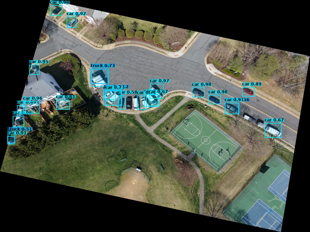
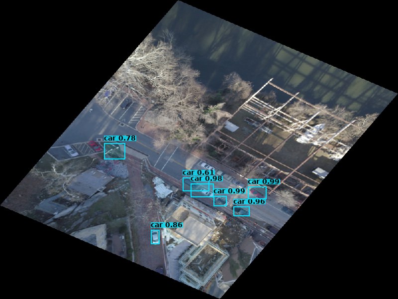
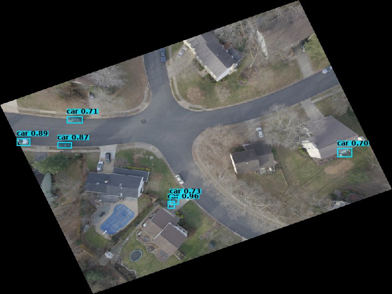
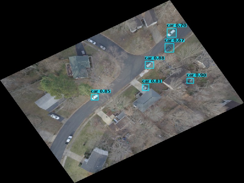
YOLO Computer Vision

Ultralytics YOLO11 running inference against COG chips fetched via TiTiler range reads. Detects vehicles, infrastructure, and activity in drone scenes — outputs geo-registered GeoJSON bounding boxes stored back into the STAC catalog.

drone_metadata_extractor · batch pipeline
YOLO11n Ultralytics COCO classes GeoJSON output
Reads COG chips via single HTTP range request — no full-scene download
Affine transform projects pixel boxes to lon/lat WGS-84 coordinates
Detection results saved as *_detections.geojson per STAC Item
Feeds spectra-enrich which writes scene labels back to the catalog
Sample detections.geojson
🧠
 PIPELINE

spectra-enrich

Enrichment pipeline that reads drone imagery through a Vision AI fallback chain, writes structured semantic metadata into STAC Items, embeds the text, and indexes vectors into Qdrant — powering hybrid search across the catalog.

spectra-enrich · batch enrichment pipeline
Claude Opus 4.5 nomic-embed-text Qdrant 768-dim vectors
Vision AI reads thumbnail → overview → COG fallback chain per item
Writes spectra:ai fields: description, scene_type, activity_level, features
Embeds enriched text via Ollama nomic-embed-text-v1.5 (sentence-transformers CPU fallback)
Upserts 768-dim Cosine vectors + metadata payload to Qdrant spectra-stac collection